If My Data Is Log10 Normal, Which Family to Use in a Glm
Modeling in R
The purpose of a statistical model is to help empathise what variables might best predict a phenomenon of interest, which ones have more or less influence, define a predictive equation with coefficients for each of the variables, and then apply that equation to predict values using the same input variables for other areas. This process requires samples with observations of the explanatory (or contained) and response (or dependent) variables in question.
We'll start with a simple linear model using our Sierra February climate information to model temperature (response variable) as predicted by elevation (explanatory variable):
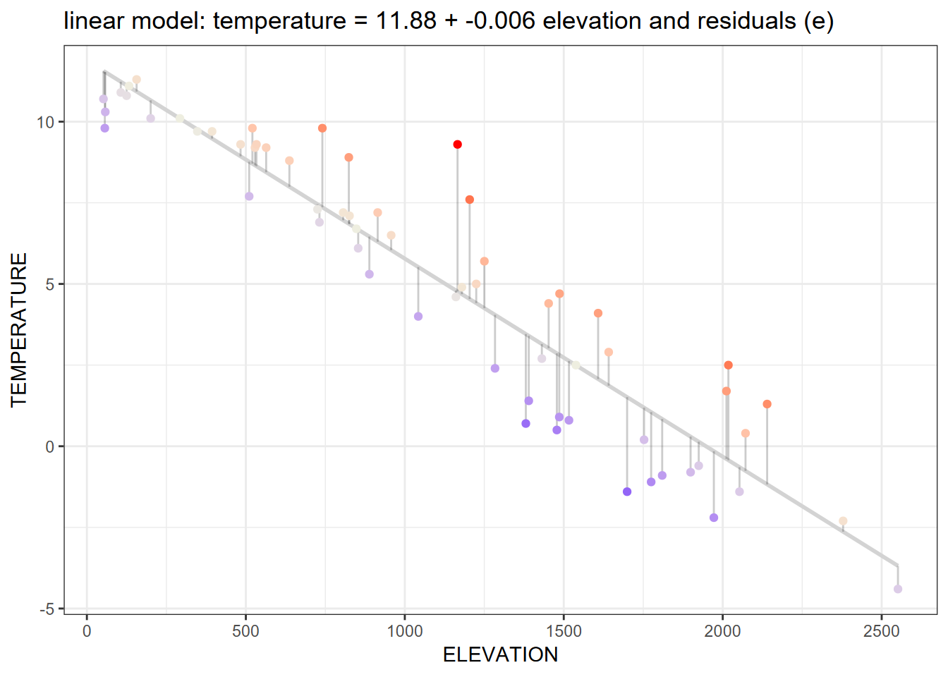
Figure 11.1: Linear model
Some common statistical models
There are many types of statistical models. Variables may be nominal (chiselled) or interval/ratio data. Yous may be interested in predicting a continuous interval/ratio variable from other continuous variables, or predicting the probability of an occurrence (eastward.g. of a species), or maybe the count of something (likewise perhaps a species). You may be needing to classify your phenomena based on continuous variables. Here are some examples:
-
lm(y ~ x)linear regression model with ane explanatory variable -
lm(y ~ x1 + x2 + x3)multiple regression, a linear model with multiple explanatory variables -
glm(y ~ ten, family = poisson)generalized linear model, poisson distribution; come across ?family unit to see those supported, including binomial, gaussian, poisson, etc. -
glm(y ~ x + y, family = binomial)glm for logistic regression -
aov(y ~ x)analysis of variance (same as lm except in the summary) -
gam(y ~ x)generalized additive models -
tree(y ~ ten)orrpart(y ~ 10)regression/nomenclature trees
Linear model (lm)
If nosotros look at the Sierra February climate instance, the regression line in the graph higher up shows the response variable temperature predicted past the explanatory variable elevation. Here's the code that produced the model and graph:
library(igisci); library(tidyverse) sierra <- sierraFeb %>% filter(! is.na(TEMPERATURE)) model1 = lm(TEMPERATURE ~ Tiptop, data = sierra) cc = model1$coefficients sierra$resid = resid(model1) sierra$predict = predict(model1) eqn = paste("temperature =", (round(cc[one], digits= two)), "+", (round(cc[2], digits= three)), "tiptop + e") ggplot(sierra, aes(ten=Peak, y=TEMPERATURE)) + geom_smooth(method= "lm", se= FALSE, color= "lightgrey") + geom_segment(aes(xend=Peak, yend=predict), blastoff=.2) + geom_point(aes(colour=resid)) + scale_color_gradient2(low= "blueish", mid= "ivory2", high= "red") + guides(color= "none") + theme_bw() + ggtitle(paste("Residuals (e) from model: ",eqn)) The summary() role can be used to look at the results statistically:
## ## Call: ## lm(formula = TEMPERATURE ~ ELEVATION, data = sierra) ## ## Residuals: ## Min 1Q Median 3Q Max ## -ii.9126 -1.0466 -0.0027 0.7940 4.5327 ## ## Coefficients: ## Approximate Std. Error t value Pr(>|t|) ## (Intercept) 11.8813804 0.3825302 31.06 <2e-16 *** ## ELEVATION -0.0061018 0.0002968 -20.56 <2e-16 *** ## --- ## Signif. codes: 0 '***' 0.001 '**' 0.01 '*' 0.05 '.' 0.ane ' ' ane ## ## Residual standard error: i.533 on sixty degrees of freedom ## Multiple R-squared: 0.8757, Adjusted R-squared: 0.8736 ## F-statistic: 422.half-dozen on 1 and threescore DF, p-value: < ii.2e-sixteen Probably the near important statistic is the p value for the explanatory variable Meridian, which in this case is very small: \(<2.2\times10^{-16}\).
The graph shows non only the linear prediction line, but also the scatter plot of input points displayed with connecting offsets indicating the magnitude of the residuum (error term) of the data point away from the prediction.
Making Predictions
Nosotros tin can use the linear equation and the coefficients derived for the intercept and the explanatory variable (and rounded a bit) to predict temperatures given the explanatory variable pinnacle, and then:
\[ Temperature_{prediction} = 11.88 - 0.006{elevation} \]
So with these coefficients, we can use the equation to a vector of elevations to predict temperature from those elevations:
a <- model1$coefficients[1] b <- model1$coefficients[2] elevations <- c(500, k, 1500, 2000) elevations ## [1] 500 thousand 1500 2000 tempEstimate <- a + b * elevations tempEstimate ## [1] viii.8304692 5.7795580 two.7286468 -0.3222645 Next, nosotros'll plot predictions and residuals on a map.
Spatial Influences on Statistical Analysis
Spatial statistical analysis brings in the spatial dimension to a statistical analysis, ranging from visual assay of patterns to specialized spatial statistical methods. There are many applications for these methods in environmental enquiry, since spatial patterns are by and large highly relevant. We might ask:
- What patterns tin we meet?
- What is the effect of scale?
- Relationships amidst variables – practise they vary spatially?
In addition to helping to identify variables not considered in the model, the effect of local weather and trend of nearby observations to be related is rich for further exploration. Readers are encouraged to larn more most spatial statistics, and some methods are explored in Hijmans (northward.d.).
But we'll utilise a fairly straightforward method that can help enlighten u.s. about the result of other variables and the influence of proximity – mapping residuals. Mapping residuals is ofttimes enlightening since they can illustrate the influence of other variables. In that location's fifty-fifty a recent weblog on this: https://californiawaterblog.com/2021/10/17/sometimes-studying-the-variation-is-the-interesting-thing/?fbclid=IwAR1tfnj2SM_du6-jEd9h-AApRPO7w88TiPUbvTFz5dkagpQ1RMV04ZZYAr8
Mapping Residuals
If we start with a map of Feb temperatures in the Sierra and endeavour to model these as predicted past elevation, we might see the following result. (First we'll build the model again, though this is probably still in retention.)
library(tidyverse) library(igisci) library(sf) sierra <- st_as_sf(filter(sierraFeb, ! is.na(TEMPERATURE)), coords= c("LONGITUDE", "LATITUDE"), crs= 4326) modelElev <- lm(TEMPERATURE ~ ELEVATION, information = sierra) summary(modelElev) ## ## Call: ## lm(formula = TEMPERATURE ~ ELEVATION, data = sierra) ## ## Residuals: ## Min 1Q Median 3Q Max ## -2.9126 -one.0466 -0.0027 0.7940 4.5327 ## ## Coefficients: ## Estimate Std. Mistake t value Pr(>|t|) ## (Intercept) 11.8813804 0.3825302 31.06 <2e-16 *** ## Pinnacle -0.0061018 0.0002968 -twenty.56 <2e-16 *** ## --- ## Signif. codes: 0 '***' 0.001 '**' 0.01 '*' 0.05 '.' 0.1 ' ' 1 ## ## Residual standard error: 1.533 on 60 degrees of freedom ## Multiple R-squared: 0.8757, Adjusted R-squared: 0.8736 ## F-statistic: 422.6 on 1 and 60 DF, p-value: < 2.2e-16 We can see from the model summary that Top is significant equally a predictor for TEMPERATURE, with a very low P value, and the R-squared value tells united states of america that 87% of the variation in temperature might be "explained" by meridian. We'll store the residuum (resid) and prediction (predict), and set up our mapping environment to create maps of the original data, prediction, and residuals.
cc <- modelElev$coefficients sierra$resid <- resid(modelElev) sierra$predict <- predict(modelElev) eqn = paste("temperature =", (round(cc[1], digits= two)), "+", (round(cc[2], digits= three)), "pinnacle") ct <- st_read(system.file("extdata","sierra/CA_places.shp",package= "igisci")) ct$AREANAME_pad <- paste0(str_replace_all(ct$AREANAME, '[A-Za-z]',' '), ct$AREANAME) bounds <- st_bbox(sierra) The original information
library(tmap); library(terra); library(igisci) hillsh <- rast(ex("CA/ca_hillsh_WGS84.tif")) tm_shape(hillsh, bbox=bounds) + tm_raster(palette= "-Greys", way= "cont", legend.show=F) + tm_shape(st_make_valid(CA_counties)) + tm_borders() + tm_shape(ct) + tm_dots() + tm_text("AREANAME", size= 0.5, only= c("left","top")) + tm_shape(sierra) + tm_symbols(col= "TEMPERATURE", palette= "-RdBu", size= 0.5) + tm_layout(legend.position= c("correct","top")) + tm_graticules(lines=F) + tm_layout(main.championship= "February Normals", principal.title.position = c("correct"), chief.title.size = 0.viii) 
Figure 11.two: Original February temperature data
The prediction map
library(tmap) tm_shape(hillsh, bbox=bounds) + tm_raster(palette= "-Greys", style= "cont", legend.show=F) + tm_shape(st_make_valid(CA_counties)) + tm_borders() + tm_shape(ct) + tm_dots() + tm_text("AREANAME", size= 0.v, just= c("left","pinnacle")) + tm_shape(sierra) + tm_symbols(col= "predict", palette= "-RdBu", size= 0.5) + tm_layout(legend.position= c("right","top")) + tm_graticules(lines=F) + tm_layout(main.title=eqn, main.title.position = c("correct"), chief.championship.size = 0.8) 
Effigy 11.iii: Temperature predicted by top model
We can also use the model to predict temperatures from a raster of elevations, which should match the elevations at the weather condition stations, allowing us to predict temperature for the remainder of the study expanse. We should have more confidence in the area (the Sierra Nevada and nearby areas) actually sampled past the stations, then we'll crop with the extent roofing that surface area (though this will include more than coastal areas that are probable to differ in Feb temperatures from patterns observed in the surface area sampled).
We'll use GCS pinnacle raster information.
library(igisci) library(tmap); library(terra) elev <- rast(ex("CA/ca_elev_WGS84.tif")) elevSierra <- crop(elev, ext(- 122, - 118, 35, 41)) # GCS b0 <- coef(modelElev)[one] b1 <- coef(modelElev)[2] tempSierra <- b0 + b1 * elevSierra names(tempSierra) = "Predicted Temperature" #tempCA <- b0 + b1 * elev tm_shape(tempSierra) + tm_raster(palette= "-RdBu") + tm_graticules(lines=F) + tm_legend(position = c("correct", "summit")) + tm_shape(st_make_valid(CA_counties)) + tm_borders() + tm_shape(ct) + tm_dots() + tm_text("AREANAME", size= 0.5, just= c("left","top")) + tm_layout(primary.title=eqn, main.title.position = c("correct"), principal.title.size = 0.7) 
Figure 11.4: Temperature predicted by summit raster
The residuals
library(tmap) tm_shape(hillsh, bbox=bounds) + tm_raster(palette= "-Greys", manner= "cont", fable.show=F) + tm_shape(st_make_valid(CA_counties)) + tm_borders() + tm_shape(ct) + tm_dots() + tm_text("AREANAME", size= 0.5, just= c("left","pinnacle")) + tm_shape(sierra) + tm_symbols(col= "resid", palette= "-RdBu", size= 0.five) + tm_layout(legend.position= c("correct","tiptop"), chief.championship = paste("east from",eqn,"+ e"), master.championship.size = 0.7, chief.title.position = "correct") + tm_graticules(lines=F) 
Figure xi.five: Residuals
Statistically, if the residuals from regression are spatially autocorrelated, we should look for patterns in the residuals to find other explanatory variables. Notwithstanding nosotros can visually see, based upon the design of the residuals, that there's at least 1 important explanatory variable not included in the model: latitude. We'll exit that for you to look at in the exercises.
Analysis of Covariance
Analysis of Covariance, or ANCOVA, has the aforementioned purpose as Analysis of Variance that we looked at nether tests earlier, just too takes into business relationship the influence of other variables called covariates. In this way, analysis of covariance combines a linear model with an analysis of variance.
"Are water samples from streams draining sandstone, limestone, and shale different based on carbonate solutes, while taking into account top?"
Response variable is modeled from the factor (ANOVA) plus the covariate (regression)
-
ANOVA:
Thursday ~ rocktype\[where TH is full hardness, a measure out of carbonate solutes\] -
Regression:
Th ~ elevation -
ANCOVA:
TH ~ rocktype + elevation- However shouldn't involve interaction betwixt
rocktype(gene) andtiptop(covariate):
- However shouldn't involve interaction betwixt
Case: stream types distinguished by discharge and gradient
Iii common river types are meandering, braided and anastomosed. For each, their slope varies by bankfull discharge in a relationship that looks something like:
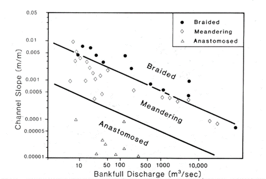
Figure 11.half dozen: Slope by Q, river types
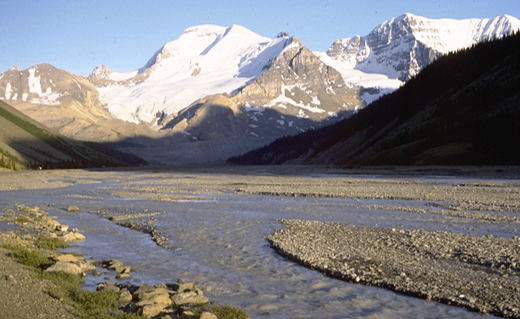
Effigy xi.7: Braided river
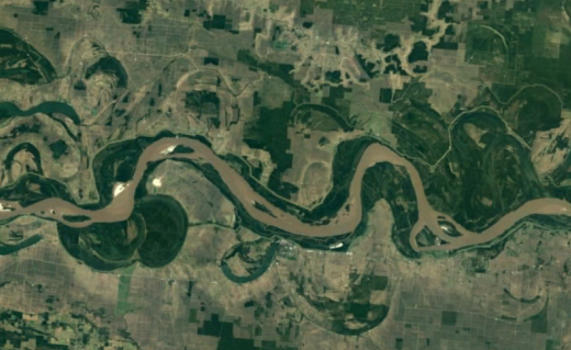
Figure 11.8: Meandering river
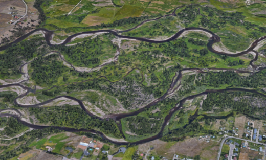
Effigy 11.9: Anastomosed river
Requirements:
- No relationship between discharge (covariate) and channel type (factor).
- Another interpretation: the gradient of the human relationship between the covariate and response variable is nearly the same for each group; simply the intercept differs. Assumes parallel slopes.
log10(Due south) ~ strtype * log10(Q) … interaction between covariate and factor
log10(South) ~ strtype + log10(Q) … no interaction, parallel slopes
If models are not significantly different, remove interaction term due to parsimony, and satisfies this ANCOVA requirement.
library(tidyverse) csvPath <- organisation.file("extdata","streams.csv", parcel= "igisci") streams <- read_csv(csvPath) streams$strtype <- gene(streams$type, labels= c("Anastomosing","Braided","Meandering")) summary(streams) ## blazon Q South strtype ## Length:41 Min. : 6 Min. :0.000011 Anastomosing: 8 ## Class :grapheme 1st Qu.: xv 1st Qu.:0.000100 Braided :12 ## Mode :character Median : twoscore Median :0.000700 Meandering :21 ## Mean : 4159 Mean :0.001737 ## 3rd Qu.: 550 3rd Qu.:0.002800 ## Max. :100000 Max. :0.009500 ggplot(streams, aes(Q, S, colour=strtype)) + geom_point() 
Figure 11.10: Q vs S: needs log scaling
library(scales) # needed for the trans_format function below ggplot(streams, aes(Q, S, color=strtype)) + geom_point() + geom_smooth(method= "lm", se = FALSE) + scale_x_continuous(trans= log10_trans(), labels = trans_format("log10", math_format(10 ^.ten))) + scale_y_continuous(trans= log10_trans(), labels = trans_format("log10", math_format(10 ^.x))) 
Figure 11.11: log scaled Q vs S with stream type
ancova = lm(log10(S)~strtype* log10(Q), data=streams) summary(ancova) ## ## Call: ## lm(formula = log10(Southward) ~ strtype * log10(Q), information = streams) ## ## Residuals: ## Min 1Q Median 3Q Max ## -0.63636 -0.13903 -0.00032 0.12652 0.60750 ## ## Coefficients: ## Estimate Std. Fault t value Pr(>|t|) ## (Intercept) -3.91819 0.31094 -12.601 1.45e-14 *** ## strtypeBraided two.20085 0.35383 6.220 three.96e-07 *** ## strtypeMeandering i.63479 0.33153 4.931 one.98e-05 *** ## log10(Q) -0.43537 0.18073 -2.409 0.0214 * ## strtypeBraided:log10(Q) -0.01488 0.19102 -0.078 0.9384 ## strtypeMeandering:log10(Q) 0.05183 0.18748 0.276 0.7838 ## --- ## Signif. codes: 0 '***' 0.001 '**' 0.01 '*' 0.05 '.' 0.1 ' ' 1 ## ## Rest standard error: 0.2656 on 35 degrees of freedom ## Multiple R-squared: 0.9154, Adjusted R-squared: 0.9033 ## F-statistic: 75.73 on 5 and 35 DF, p-value: < 2.2e-16 ## Assay of Variance Table ## ## Response: log10(Southward) ## Df Sum Sq Mean Sq F value Pr(>F) ## strtype ii 18.3914 ix.1957 130.3650 < 2.2e-xvi *** ## log10(Q) 1 8.2658 eight.2658 117.1821 1.023e-12 *** ## strtype:log10(Q) 2 0.0511 0.0255 0.3619 0.6989 ## Residuals 35 2.4688 0.0705 ## --- ## Signif. codes: 0 '***' 0.001 '**' 0.01 '*' 0.05 '.' 0.1 ' ' 1 # At present an additive model, which does not have that interaction ancova2 = lm(log10(S)~strtype+ log10(Q), information=streams) anova(ancova2) ## Analysis of Variance Table ## ## Response: log10(Due south) ## Df Sum Sq Mean Sq F value Pr(>F) ## strtype 2 18.3914 9.1957 135.02 < 2.2e-16 *** ## log10(Q) i 8.2658 8.2658 121.37 3.07e-xiii *** ## Residuals 37 ii.5199 0.0681 ## --- ## Signif. codes: 0 '***' 0.001 '**' 0.01 '*' 0.05 '.' 0.1 ' ' 1 ## Analysis of Variance Table ## ## Model 1: log10(S) ~ strtype * log10(Q) ## Model 2: log10(South) ~ strtype + log10(Q) ## Res.Df RSS Df Sum of Sq F Pr(>F) ## 1 35 two.4688 ## 2 37 2.5199 -two -0.051051 0.3619 0.6989 # not significantly different, so model simplification is justified # Now we remove the strtype term ancova3 = update(ancova2, ~ . - strtype) anova(ancova2,ancova3) ## Assay of Variance Table ## ## Model one: log10(S) ~ strtype + log10(Q) ## Model 2: log10(S) ~ log10(Q) ## Res.Df RSS Df Sum of Sq F Pr(>F) ## 1 37 ii.5199 ## 2 39 25.5099 -2 -22.99 168.78 < ii.2e-16 *** ## --- ## Signif. codes: 0 '***' 0.001 '**' 0.01 '*' 0.05 '.' 0.1 ' ' ane # Goes too far. Removing the strtype creates a significantly different model step(ancova) ## Start: AIC=-103.2 ## log10(S) ~ strtype * log10(Q) ## ## Df Sum of Sq RSS AIC ## - strtype:log10(Q) two 0.051051 2.5199 -106.36 ## <none> 2.4688 -103.20 ## ## Stride: AIC=-106.36 ## log10(S) ~ strtype + log10(Q) ## ## Df Sum of Sq RSS AIC ## <none> 2.5199 -106.364 ## - log10(Q) 1 viii.2658 ten.7857 -48.750 ## - strtype 2 22.9901 25.5099 -15.455 ## ## Call: ## lm(formula = log10(S) ~ strtype + log10(Q), information = streams) ## ## Coefficients: ## (Intercept) strtypeBraided strtypeMeandering log10(Q) ## -three.9583 2.1453 i.7294 -0.4109 ANOVA & ANCOVA are applications of a linear model.
- Uses lm in R
- Response variable is continuous, assumed normally distributed
mymodel = lm(log10(S) ~ strtype + log10(Q))
- The linear model, with categorical explanatory variable + covariate
anova(mymodel)
- Displays the Analysis of Variance table from the linear model
Generalized Linear Model (GLM)
The glm in R allows you to work with diverse types of information using various distributions, described as families such as:
-
gaussian: normal distribution – what is used with lm -
binomial: logit – used with probabilities.- Used for logistic regression
- A simple instance of predicting a canis familiaris panting or not (a binomial, since the dog either panted or didn't) related to temperature: https://bscheng.com/2016/10/23/logistic-regression-in-r/
-
poisson: for counts. Unremarkably used for species counts. -
see
help(glm)for other examples
Binomial family: Logistic GLM with streams
When the glm family unit is binomial, nosotros might exercise what's sometimes chosen logistic regression where we look at the probability of a categorical value (might be a species occurrence, for instance) given various independent variables. Let'southward try this with the streams data nosotros simply used for analysis of covariance, to predict the probability of a item stream type from slope and discharge:
library(igisci) library(tidyverse) streams <- read_csv(ex("streams.csv")) streams$strtype <- factor(streams$type, labels= c("Anastomosing","Braided","Meandering")) For logistic regression, nosotros demand probability data, so locations where nosotros know the probability of something being truthful. If you think nigh it, that'due south pretty difficult to know for an ascertainment, but we might know whether something is true or not, similar we observed the phenomenon or not, and so nosotros simply assign a probability of i if something is observed, and 0 if information technology'southward not. Since in the case of the stream types, we really take iii unlike probabilities: whether it's truthful that the stream is anastomosing, whether it's braided and whether information technology's meandering, and then we'll create three dummy variables for that with values of 1 or 0: if information technology'southward braided, the value for braided is i, otherwise information technology'south 0; the same applies to all 3 dummy variables:
streams <- streams %>% mutate(braided = ifelse(type == "B", 1, 0), meandering = ifelse(type == "G", one, 0), anastomosed = ifelse(type == "A", 1, 0)) streams ## # A tibble: 41 x vii ## blazon Q S strtype braided meandering anastomosed ## <chr> <dbl> <dbl> <fct> <dbl> <dbl> <dbl> ## 1 B 9.9 0.0045 Braided 1 0 0 ## 2 B 11 0.007 Braided one 0 0 ## 3 B xvi 0.0068 Braided 1 0 0 ## 4 B 25 0.0042 Braided 1 0 0 ## 5 B 40 0.0028 Braided 1 0 0 ## 6 B 150 0.0041 Braided one 0 0 ## 7 B 190 0.002 Braided one 0 0 ## 8 B 550 0.0007 Braided 1 0 0 ## ix B 1100 0.00055 Braided i 0 0 ## 10 B 7100 0.00042 Braided 1 0 0 ## # ... with 31 more rows So nosotros tin run the logistic regression on each one:
summary(glm(braided ~ log(Q) + log(S), family=binomial, data=streams)) ## ## Call: ## glm(formula = braided ~ log(Q) + log(S), family = binomial, data = streams) ## ## Deviance Residuals: ## Min 1Q Median 3Q Max ## -2.00386 -0.49007 -0.00961 0.15789 1.58088 ## ## Coefficients: ## Estimate Std. Error z value Pr(>|z|) ## (Intercept) 17.5853 6.7443 2.607 0.00912 ** ## log(Q) 2.0940 0.8135 2.574 0.01005 * ## log(S) 4.3115 ane.6173 two.666 0.00768 ** ## --- ## Signif. codes: 0 '***' 0.001 '**' 0.01 '*' 0.05 '.' 0.ane ' ' one ## ## (Dispersion parameter for binomial family taken to exist ane) ## ## Naught deviance: 49.572 on 40 degrees of freedom ## Balance deviance: 23.484 on 38 degrees of freedom ## AIC: 29.484 ## ## Number of Fisher Scoring iterations: 8 summary(glm(meandering ~ log(Q) + log(S), family=binomial, information=streams)) ## ## Call: ## glm(formula = meandering ~ log(Q) + log(Southward), family = binomial, ## data = streams) ## ## Deviance Residuals: ## Min 1Q Median 3Q Max ## -1.5469 -i.2515 0.8197 one.1073 1.3072 ## ## Coefficients: ## Estimate Std. Error z value Pr(>|z|) ## (Intercept) 2.43255 1.38078 ane.762 0.0781 . ## log(Q) 0.04984 0.13415 0.372 0.7103 ## log(Due south) 0.34750 0.19471 ane.785 0.0743 . ## --- ## Signif. codes: 0 '***' 0.001 '**' 0.01 '*' 0.05 '.' 0.ane ' ' 1 ## ## (Dispersion parameter for binomial family taken to be 1) ## ## Null deviance: 56.814 on 40 degrees of freedom ## Residual deviance: 53.074 on 38 degrees of freedom ## AIC: 59.074 ## ## Number of Fisher Scoring iterations: iv summary(glm(anastomosed ~ log(Q) + log(Southward), family=binomial, information=streams)) ## ## Call: ## glm(formula = anastomosed ~ log(Q) + log(Due south), family = binomial, ## data = streams) ## ## Deviance Residuals: ## Min 1Q Median 3Q Max ## -two.815e-05 -2.110e-08 -2.110e-08 -2.110e-08 2.244e-05 ## ## Coefficients: ## Estimate Std. Fault z value Pr(>|z|) ## (Intercept) -176.09 786410.69 0 1 ## log(Q) -11.81 77224.35 0 1 ## log(South) -24.18 70417.40 0 1 ## ## (Dispersion parameter for binomial family taken to be one) ## ## Nothing deviance: four.0472e+01 on 40 degrees of liberty ## Residue deviance: 1.3027e-09 on 38 degrees of freedom ## AIC: 6 ## ## Number of Fisher Scoring iterations: 25 So what we can see from this admittedly pocket-size sample is that:
- Predicting braided character from Q and S works pretty well, distinguishing these characteristics from the characteristics of all other streams \[`braided==0`\]
- Predicting anastomosed or meandering however isn't pregnant.
We really need a larger sample size, and Due north American geomorphology has recently discovered the "anabranching" stream type (of which anastomosed is a type) that had been long recognized in Commonwealth of australia, and its characteristics range across meandering at to the lowest degree, then muddying the waters…
Logistic landslide model
With its active tectonics, steep slopes and relatively common intense rain events during the wintertime season, littoral California has a propensity for landslides. Pacifica has been the focus of many landslide studies by the USGS and others, with events ranging from coastal erosion influenced by wave action to landslides and debris flows on steep hillslopes driven by positive pore force per unit area (Ellen and Wieczorek (1988)).
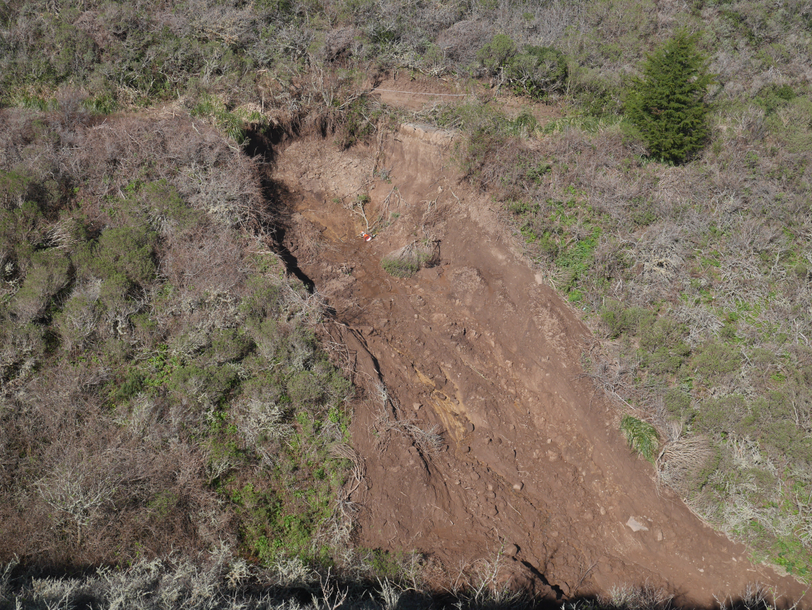
Figure 11.12: Landslide in San Pedro Creek watershed
Figure 11.13: Sediment source analysis
Also encounter the relevant department in the San Pedro Creek Virtual Fieldtrip story map: J. Davis (n.d.).
Landslides detected in San Pedro Creek Watershed in Pacifica, CA, are in the SanPedro folder of extdata. Landslides were detected on aerial photography from 1941, 1955, 1975, 1983, and 1997, and confirmed in the field during a study in the early 2000's (Sims (2004), J. Davis and Blesius (2015)). We'll create a logistic regression to compare landslide probability to various ecology factors. We'll use elevation, slope and other derivatives, distance to streams, distance to trails, and the results of a physical model predicting gradient stability every bit a stability alphabetize (SI), using slope and soil transmissivity data.
library(igisci); library(sf); library(tidyverse); library(terra) slides <- st_read(ex("SanPedro/slideCentroids.shp")) %>% mutate(IsSlide = 1) slides$Visible <- factor(slides$Visible) trails <- st_read(ex("SanPedro/trails.shp")) streams <- st_read(ex("SanPedro/streams.shp")) wshed <- st_read(ex("SanPedro/SPCWatershed.shp")) ggplot(information=slides) + geom_sf(aes(col=Visible)) + scale_color_brewer(palette= "Spectral") + geom_sf(data=streams, col= "blue") + geom_sf(data=wshed, fill up= NA) 
Figure 11.xiv: Landslides in San Pedro Creek watershed
At this point, we take data for occurrences of landslides, and so for each point we assign the dummy variable IsSlide = 1. We don't have any absence data, simply we can create some using random points and assign them IsSlide = 0. Information technology would probably exist a adept idea to avoid areas very close to the occurrences, simply nosotros'll just put random points everywhere and only remove the ones that don't have SI data.
For the random locations, we'll set a seed and then for the book the results will stay the same; and if we're adept with that since it doesn't actually thing what seed we apply, we might besides use the answer to everything: 42.
library(terra) elev <- rast(ex("SanPedro/dem.tif")) SI <- rast(ex("SanPedro/SI.tif")) npts <- length(slides$Visible) * ii # up information technology a little to become plenty afterward clip set.seed(42) ten <- runif(npts, min= xmin(elev), max= xmax(elev)) y <- runif(npts, min= ymin(elev), max= ymax(elev)) rsampsRaw <- st_as_sf(data.frame(ten,y), coords = c("10","y"), crs= crs(elev)) ggplot(data=rsampsRaw) + geom_sf(size= 0.five) + geom_sf(data=streams, col= "blue") + geom_sf(data=wshed, fill= NA) 
Figure 11.fifteen: Raw random points
At present we accept twice as many random points as we take landslides, within the rectangular extend of the watershed, as defined by the elevation raster. Nosotros doubled these because we need to exclude some points, yet still have enough to be roughly as many random points as slides. We'll exclude:
- all points outside the watershed
- points within 100 m of the landslide occurrences, the distance based on knowledge of the grain of landscape features (like spurs and swales) that might influence landslide occurrence
slideBuff <- st_buffer(slides, 100) wshedNoSlide <- st_difference(wshed, st_union(slideBuff)) The 100 m buffer excludes all areas around all landslides in the data set up. We're going to run the model on specific years, but the all-time option of landslide absences will be to exclude areas around all landslides we know of.
ggplot(data=slides) + geom_sf(aes(col=Visible)) + scale_color_brewer(palette= "Spectral") + geom_sf(data=streams, col= "blue") + geom_sf(information=wshedNoSlide, fill= NA) 
Figure eleven.16: Landslides and buffers to exclude from random points
rsamps <- st_intersection(rsampsRaw,wshedNoSlide) %>% mutate(IsSlide = 0) allPts <- bind_rows(slides, rsamps) ggplot(data=allPts) + geom_sf(aes(col=IsSlide)) + geom_sf(data=streams, col= "blue") + geom_sf(data=wshed, make full= NA) 
Figure 11.17: Landslides and random points (excluded from slide buffers)
Now we'll derive some environmental variables as rasters and extract their values to the slide/noslide bespeak information set. We'll use the shade function to create an exposure raster with the lord's day at the boilerplate noon angle from the southward. Notation the utilise of dplyr::rename to create meaningful variable names for rasters that had names like "lyr1" (who knows why?) which I determined past running information technology without the rename and seeing what information technology produced.
slidesV <- vect(allPts) strms <- rasterize(vect(streams),elev) tr <- rasterize(vect(trails),elev) stD <- altitude(strms); names(stD) = "stD" trD <- distance(tr); names(trD) = "trD" gradient <- terrain(elev, v= "slope") curv <- terrain(slope, v= "slope") aspect <- terrain(elev, v= "aspect") exposure <- shade(slope/ 180 *pi,aspect/ 180 *pi,angle= 53,direction= 180) elev_ex <- terra:: excerpt(elev, slidesV) %>% rename(elev=dem) %>% dplyr:: select(-ID) SI_ex <- terra:: excerpt(SI, slidesV) %>% dplyr:: select(-ID) slope_ex <- terra:: extract(slope, slidesV) %>% dplyr:: select(-ID) curv_ex <- terra:: extract(curv, slidesV) %>% rename(curv = slope) %>% dplyr:: select(-ID) exposure_ex <- terra:: extract(exposure, slidesV) %>% rename(exposure=lyr1) %>% dplyr:: select(-ID) stD_ex <- terra:: extract(stD, slidesV) %>% dplyr:: select(-ID) trD_ex <- terra:: extract(trD, slidesV) %>% dplyr:: select(-ID) slidePts <- cbind(allPts,elev_ex,SI_ex,slope_ex,curv_ex,exposure_ex,stD_ex,trD_ex) slidesData <- every bit.data.frame(slidePts) %>% filter(! is.nan(SI)) %>% st_as_sf(crs= st_crs(slides)) We'll filter for just the slides in the 1983 imagery, and for the model also include all of the random points (detected with NA values for Visible):
slides83 <- slidesData %>% filter(Visible == 1983) slides83plusr <- slidesData %>% filter(Visible == 1983 | is.na(Visible)) The logistic regression in the glm model uses the binomial family:
summary(glm(IsSlide ~ SI + curv + elev + slope + exposure + stD + trD, family=binomial, data=slides83plusr)) ## ## Call: ## glm(formula = IsSlide ~ SI + curv + elev + slope + exposure + ## stD + trD, family = binomial, information = slides83plusr) ## ## Deviance Residuals: ## Min 1Q Median 3Q Max ## -2.3819 -0.5882 -0.0002 0.7378 3.9146 ## ## Coefficients: ## Guess Std. Error z value Pr(>|z|) ## (Intercept) 0.1426071 1.0618610 0.134 0.89317 ## SI -i.8190286 0.3639202 -4.998 5.78e-07 *** ## curv 0.0059237 0.0113657 0.521 0.60223 ## elev -0.0025050 0.0014398 -1.740 0.08190 . ## gradient 0.0623201 0.0211010 2.953 0.00314 ** ## exposure ii.6971912 0.6603844 4.084 4.42e-05 *** ## stD -0.0052639 0.0019765 -2.663 0.00774 ** ## trD -0.0020730 0.0006532 -three.174 0.00150 ** ## --- ## Signif. codes: 0 '***' 0.001 '**' 0.01 '*' 0.05 '.' 0.ane ' ' i ## ## (Dispersion parameter for binomial family taken to be 1) ## ## Null deviance: 668.29 on 483 degrees of freedom ## Residual deviance: 402.90 on 476 degrees of freedom ## AIC: 418.9 ## ## Number of Fisher Scoring iterations: 8 So while we might want to make certain that we've picked the right variables, some conclusions from this might be that stability index (SI) is non surprisingly a strong predictor of landslides, only also that other than elevation and curvature, the other variables are also pregnant.
Map the logistic effect
Should exist able to, but need to use the formula for the model, which in our case volition have half-dozen explanatory variables SI (\(X_1\)), elev (\(X_2\)), gradient (\(X_3\)), exposure (\(X_4\)), stD (\(X_5\)) and trD (\(X_6\)): \[p = \frac{e^{b_0+b_1X_1+b_2X_2+b_3X_3+b_4X_4+b_5X_5}}{1+e^{b_0+b_1X_1+b_2X_2+b_3X_3+b_4X_4+b_5X_5}}\]
So nosotros retrieve the coefficients with coef() and use map algebra to create the prediction map, including dots for the landslides actually observed in 1983:
library(tmap) SI_stD_model <- glm(IsSlide ~ SI + gradient + exposure + stD + trD, family=binomial, data=slides83plusr) b0 <- coef(SI_stD_model)[1] b1 <- coef(SI_stD_model)[2] b2 <- coef(SI_stD_model)[three] b3 <- coef(SI_stD_model)[4] b4 <- coef(SI_stD_model)[5] b5 <- coef(SI_stD_model)[half-dozen] predictionMap <- (exp(b0+b1*SI+b2*slope+b3*exposure+b4*stD+b5*trD))/ (1 + exp(b0+b1*SI+b2*slope+b3*exposure+b4*stD+b5*trD)) names(predictionMap) <- "slide_probability_1983" tm_shape(predictionMap) + tm_raster() + tm_shape(streams) + tm_lines(col= "blue") + tm_shape(wshed) + tm_borders(col= "blackness") + tm_shape(slides83) + tm_dots(col= "greenish") + tm_layout(title= "Predicted by SI, slope, exposure, streamD, trailD") + tm_graticules(lines=F) 
Figure 11.18: Logistic model prediction of 1983 landslide probability
Poisson regression
Poission regression (family=poisson in glm) is for analyzing counts. Yous might utilize this to determine which variables are significant predictors, or y'all might desire to see where or when counts are especially loftier, or college than expected. Or it might exist applied to compare groupings. For case, if instead of looking at differences amongst rock types in Sinking Cove based on chemical properties in h2o samples or measurements (where we applied ANOVA), we looked at differences in fish counts, that might exist an application of poisson regression, as long equally other information assumptions agree.
- An caption of poisson distribution using meteor showers at: https://towardsdatascience.com/the-poisson-distribution-and-poisson-procedure-explained-4e2cb17d459
- An explanation of poisson distribution applied to schooling data: https://stats.oarc.ucla.edu/r/dae/poisson-regression/
Seabird Poisson Model
This model is further developed in a case report where nosotros'll map a prediction, but we'll look at the basics for applying a poisson family model in glm: seabird observations. The data is potentially suitable since information technology's counts with known time intervals of observation effort and initial review of the information suggests that the mean counts is reasonably similar to the variance. The information were nerveless through the Access program ( Applied California Current Ecosystem Studies (n.d.)) and a thorough analysis provided by Studwell et al. (2017).
library(igisci); library(sf); library(tidyverse); library(tmap) library(maptiles) transects <- st_read(ex("SFmarine/transects.shp")) One of the seabirds studies, the blackness-footed albatross, has the lowest counts so a relatively rare bird, and studies of its distribution may be informative. We'll await at counts collected during transect cruises in July 2006.
tmap_mode("plot") oceanBase <- get_tiles(transects, provider= "Esri.OceanBasemap") transJul2006 <- transects %>% filter(calendar month== seven & yr== 2006 & avg_tem> 0 & avg_sal> 0 & avg_fluo> 0) tm_shape(oceanBase) + tm_rgb() + tm_shape(transJul2006) + tm_symbols(col= "bfal", size= "bfal") 
Effigy 11.xix: Black-footed albatross counts, July 2006
Prior studies have suggested that temperature, salinity, fluorescence, depth and various distances might be good explanatory variables to use to look at spatial patterns, and then we'll employ these in the model.
summary(glm(bfal~avg_tem+avg_sal+avg_fluo+avg_dep+dist_land+dist_isla+dist_200m+dist_cord, data=transJul2006,family=poisson)) ## ## Telephone call: ## glm(formula = bfal ~ avg_tem + avg_sal + avg_fluo + avg_dep + ## dist_land + dist_isla + dist_200m + dist_cord, family = poisson, ## information = transJul2006) ## ## Deviance Residuals: ## Min 1Q Median 3Q Max ## -1.2935 -0.4646 -0.2445 -0.0945 4.7760 ## ## Coefficients: ## Approximate Std. Error z value Pr(>|z|) ## (Intercept) -1.754e+02 7.032e+01 -2.495 0.01260 * ## avg_tem 7.341e-01 three.479e-01 2.110 0.03482 * ## avg_sal five.202e+00 two.097e+00 2.480 0.01312 * ## avg_fluo -six.978e-01 1.217e+00 -0.574 0.56626 ## avg_dep -iii.561e-03 viii.229e-04 -four.328 1.51e-05 *** ## dist_land -two.197e-04 6.194e-05 -3.547 0.00039 *** ## dist_isla 1.372e-05 1.778e-05 0.771 0.44043 ## dist_200m -4.696e-04 i.037e-04 -4.528 5.95e-06 *** ## dist_cord -v.213e-06 1.830e-05 -0.285 0.77570 ## --- ## Signif. codes: 0 '***' 0.001 '**' 0.01 '*' 0.05 '.' 0.1 ' ' 1 ## ## (Dispersion parameter for poisson family unit taken to be one) ## ## Null deviance: 152.14 on 206 degrees of freedom ## Residual deviance: 105.73 on 198 degrees of freedom ## AIC: 160.37 ## ## Number of Fisher Scoring iterations: 7 Nosotros can see in the model coefficients table several predictive variables that appear to exist significant, which nosotros'll explore further in the example study.
- avg_tem
- avg_sal
- avg_dep
- dist_land
- dist_200m
Note R will allow you to run glm on any family, just information technology'south upward to y'all to make sure it's appropriate. For example, if yous provide a response variable that is not count data or doesn't fit the requirements for a poisson model, R will create a result just it's bogus.
Models Employing Machine Learning
Models using machine learning algorithms are commonly used in information science, fitting with its general exploratory and data-mining approach. There are many auto learning algorithms, and many resources for learning more about them, but they all share a basically black-box approach where a collection of variables are explored for patterns in input variables that help to explicate a response variable. The latter is like to more than conventional statistical modeling depict above, with the divergence existence the machine learning approach – call back of robots going through your data looking for connections.
We'll explore a few car learning methods (such equally neural networks, random forests, and support vector machines) in a subsequently affiliate when nosotros endeavor to use them to allocate satellite imagery, an important environmental application. Equally this application is in the spatial domain, we might desire to wait further into spatial statistical methods.
Exercise
-
Start by creating a new RStudio projection "modeling" including a "data" folder we'll use for the last question when you lot bring in your own information.
-
Add together
LATITUDEas a second independent variable afterElevationin the model predicting February temperatures. Note that you'll need to change a setting in thest_as_sfto not removeLatitudeandLONGITUDE, then y'all'll need to modify thelmregression formula to include bothELEVATION + LATITUDE. Offset derive and display the model summary results, and so answer the questions – is the caption meliorate based on the \(r^2\)? -
At present map the predictions and residuals.
Figure 11.20: Goal of Question ii
-
Can you come across any potential for additional variables? What testify might there be for localized effects?
-
Let's build a prediction raster from the above model. First past reading in the
ca_elev_WGS84.tifraster equally was done before, with the same crop, and once again assigning it toelevSierra, and get the iii coefficientsb0,b1, andb2.
- Now utilise the following lawmaking to create a raster of the same dimensions as
elevSierra, but with latitude assigned as z values to the cells:
lats <- yFromCell(elevSierra, one : ncell(elevSierra)) latitude <- setValues(elevSierra,lats) plot(latitude) 
Figure 11.21: Latitude raster
- And so build a raster prediction of temperature from the model and the two explanatory rasters.

Effigy eleven.22: Goal of Question 4
-
Modify the code for the San Pedro Creek Watershed logistical model to look at 1975 landslides. Are the conclusions unlike?
-
Using your own information, that should have location data also equally other attributes, create a statistical model of your choice, and provide your assessment of the results, a prediction map, and where advisable mapped residuals.
-
Optionally, using your ain information, no location information needed, create a glm binomial model. If you don't have anything obvious, consider doing something like the study of a pet domestic dog panting based on temperature. https://bscheng.com/2016/10/23/logistic-regression-in-r/
References
Applied California Current Ecosystem Studies. due north.d. https://www.accessoceans.org.
Davis, Jerry. n.d. San Pedro Creek Watershed Virtual Fieldtrip: Story Map. https://storymaps.arcgis.com/stories/62705877a9f64ac5956a64230430c248.
Davis, Jerry, and Leonhard Blesius. 2015. "A Hybrid Physical and Maximum-Entropy Landslide Susceptibility Model." Entropy 17 (half-dozen): 4271–92. https://world wide web.mdpi.com/1099-4300/17/6/4271.
Ellen, Stephen D., and Gerald F. Wieczorek. 1988. Landslides, Floods, and Marine Furnishings of the Tempest of January 3-5, 1982, in the San Francisco Bay Region, California. Vol. 1434. USGS. https://pubs.usgs.gov/pp/1988/1434/.
Hijmans, Robert J. n.d. Spatial Data Science. https://rspatial.org.
Sims, Stephanie. 2004. Hillslope Sediment Source Cess of San Pedro Creek Watershed, California. https://geog.sfsu.edu/thesis/hillslope-sediment-source-cess-san-pedro-creek-watershed-california.
Studwell, Anna, Ellen Hines, Meredith L. Elliott, Julie Howar, Barbara Holzman, Nadav Nur, and Jaime Jahncke. 2017. "Modeling Nonresident Seabird Foraging Distributions to Inform Body of water Zoning in Key California." PLoS Ane. https://doi.org/10.1371/journal.pone.0169517.
nelsonoursend1939.blogspot.com
Source: https://bookdown.org/igisc/EnvDataSci/modeling-in-r.html
Postar um comentário for "If My Data Is Log10 Normal, Which Family to Use in a Glm"